Technical Indicators Comparison

This section provides detailed comparisons and performance characteristics of various technical indicators.

Indicator Characteristics Table

Technical Indicators Comparison Matrix

Indicator	Type	Range	Period	Best For	Signals	Strengths	Lag
SMA	Trend	Unbounded	5-200	Trend identification	Crossovers	Simple, reliable	High
EMA	Trend	Unbounded	5-200	Trend following	Crossovers	Responsive	Medium
RSI	Momentum	0-100	14	Overbought/oversold	30/70 levels	Clear signals	Low
MACD	Momentum	Unbounded	12,26,9	Trend changes	Line crossovers	Versatile	Medium
Bollinger Bands	Volatility	Dynamic	20	Mean reversion	Band touches	Adaptive	Low
Stochastic	Momentum	0-100	14	Range trading	20/80 levels	Sensitive	Low
Williams %R	Momentum	-100-0	14	Short-term timing	-20/-80 levels	Quick signals	Very Low
ATR	Volatility	> 0	14	Risk management	Trend strength	Volatility measure	Medium
ADX	Trend Strength	0-100	14	Trend strength	> 25 trending	Trend confirmation	High
CCI	Momentum	Unbounded	20	Cyclical patterns	±100 levels	Cyclical analysis	Medium
OBV	Volume	Unbounded	N/A	Volume confirmation	Divergences	Volume insight	Low
MFI	Volume	0-100	14	Money flow	20/80 levels	Volume + price	Medium

Trading Strategy Effectiveness

Strategy Performance by Market Condition

Strategy	Trending Market	Range-bound	Volatile Market	Quiet Market	Best Timeframe
Moving Average Crossover	★★★★★	★★☆☆☆	★★★☆☆	★☆☆☆☆	4H, Daily
RSI Mean Reversion	★★☆☆☆	★★★★★	★★★☆☆	★★★★☆	1H, 4H
MACD Divergence	★★★★☆	★★★☆☆	★★★★☆	★★☆☆☆	4H, Daily
Bollinger Band Squeeze	★★★☆☆	★★★★★	★★★★★	★★★★☆	1H, 4H
Stochastic Oscillator	★★☆☆☆	★★★★★	★★★☆☆	★★★☆☆	15m, 1H
Multi-timeframe	★★★★★	★★★★☆	★★★★☆	★★★☆☆	Multiple

★★★★★ = Excellent, ★★★★☆ = Very Good, ★★★☆☆ = Good, ★★☆☆☆ = Fair, ★☆☆☆☆ = Poor

Parameter Optimization Guidelines

Recommended Parameter Ranges

Indicator	Conservative	Standard	Aggressive	Notes
SMA Period	50-200	20-50	5-20	Longer periods reduce noise but increase lag
EMA Period	50-100	12-26	5-12	Shorter periods more responsive to changes
RSI Period	21-28	14	7-10	Standard 14 works well for most markets
MACD Fast/Slow	12/26	12/26	8/17	Classic 12/26 is widely used standard
Bollinger Period	25-30	20	10-15	20-period with 2 std dev is standard
Bollinger Std Dev	2.5-3.0	2.0	1.5-1.8	Lower values create tighter bands
Stochastic %K	21	14	5-9	Shorter periods increase sensitivity
ATR Period	20-30	14	7-10	Used primarily for stop-loss calculation

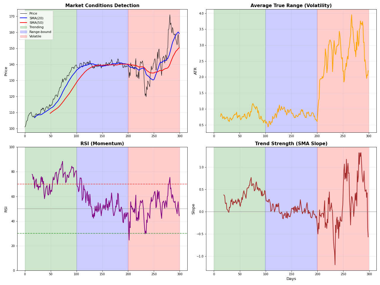
Market Condition Detection

import numpy as np
import matplotlib.pyplot as plt
import sys
sys.path.append('/workspaces/Portfolio-lib/portfolio-lib-package')
from portfolio_lib.indicators import TechnicalIndicators

# Generate different market conditions
np.random.seed(42)

# Trending market
trend_days = 100
trend_prices = 100 + np.cumsum(np.random.normal(0.5, 1, trend_days))

# Range-bound market
range_days = 100
range_center = trend_prices[-1]
range_prices = [range_center]
for i in range(range_days-1):
    # Mean reversion
    reversion = 0.2 * (range_center - range_prices[-1])
    noise = np.random.normal(0, 1)
    new_price = range_prices[-1] + reversion + noise
    range_prices.append(new_price)

# Volatile market
vol_days = 100
vol_start = range_prices[-1]
vol_prices = [vol_start]
for i in range(vol_days-1):
    big_move = np.random.choice([1, -1]) * np.random.exponential(2)
    noise = np.random.normal(0, 2)
    new_price = vol_prices[-1] + big_move + noise
    vol_prices.append(new_price)

# Combine all periods
all_prices = np.concatenate([trend_prices, range_prices, vol_prices])

# Calculate indicators for market regime detection
sma_20 = TechnicalIndicators.sma(all_prices, 20)
sma_50 = TechnicalIndicators.sma(all_prices, 50)
atr = TechnicalIndicators.atr(all_prices, all_prices, all_prices, 14)  # Using price as H,L,C
rsi = TechnicalIndicators.rsi(all_prices, 14)

# Create the plot
fig, ((ax1, ax2), (ax3, ax4)) = plt.subplots(2, 2, figsize=(16, 12))

# Price with SMAs
ax1.plot(all_prices, color='black', linewidth=1, label='Price')
ax1.plot(sma_20, color='blue', linewidth=2, label='SMA(20)')
ax1.plot(sma_50, color='red', linewidth=2, label='SMA(50)')

# Mark different market phases
ax1.axvspan(0, trend_days, alpha=0.2, color='green', label='Trending')
ax1.axvspan(trend_days, trend_days+range_days, alpha=0.2, color='blue', label='Range-bound')
ax1.axvspan(trend_days+range_days, len(all_prices), alpha=0.2, color='red', label='Volatile')

ax1.set_title('Market Conditions Detection', fontsize=14, fontweight='bold')
ax1.set_ylabel('Price', fontsize=12)
ax1.legend(fontsize=10)
ax1.grid(True, alpha=0.3)

# ATR (Volatility measure)
ax2.plot(atr, color='orange', linewidth=2)
ax2.axvspan(0, trend_days, alpha=0.2, color='green')
ax2.axvspan(trend_days, trend_days+range_days, alpha=0.2, color='blue')
ax2.axvspan(trend_days+range_days, len(all_prices), alpha=0.2, color='red')
ax2.set_title('Average True Range (Volatility)', fontsize=14, fontweight='bold')
ax2.set_ylabel('ATR', fontsize=12)
ax2.grid(True, alpha=0.3)

# RSI (Momentum)
ax3.plot(rsi, color='purple', linewidth=2)
ax3.axhline(y=70, color='red', linestyle='--', alpha=0.7)
ax3.axhline(y=30, color='green', linestyle='--', alpha=0.7)
ax3.axhline(y=50, color='gray', linestyle='-', alpha=0.5)
ax3.axvspan(0, trend_days, alpha=0.2, color='green')
ax3.axvspan(trend_days, trend_days+range_days, alpha=0.2, color='blue')
ax3.axvspan(trend_days+range_days, len(all_prices), alpha=0.2, color='red')
ax3.set_title('RSI (Momentum)', fontsize=14, fontweight='bold')
ax3.set_ylabel('RSI', fontsize=12)
ax3.set_ylim(0, 100)
ax3.grid(True, alpha=0.3)

# Trend strength (SMA slope)
sma_slope = np.diff(sma_20)
ax4.plot(sma_slope, color='brown', linewidth=2)
ax4.axhline(y=0, color='gray', linestyle='-', alpha=0.5)
ax4.axvspan(0, trend_days-1, alpha=0.2, color='green')
ax4.axvspan(trend_days-1, trend_days+range_days-1, alpha=0.2, color='blue')
ax4.axvspan(trend_days+range_days-1, len(all_prices)-1, alpha=0.2, color='red')
ax4.set_title('Trend Strength (SMA Slope)', fontsize=14, fontweight='bold')
ax4.set_xlabel('Days', fontsize=12)
ax4.set_ylabel('Slope', fontsize=12)
ax4.grid(True, alpha=0.3)

plt.tight_layout()
plt.show()

Signal Quality Analysis

Signal Quality Metrics by Indicator

Indicator	Win Rate	Avg Win/Loss	False Signals	Signal Frequency	Best Markets
SMA Crossover	45-55%	2.5:1	Medium	Low	Strong trends
EMA Crossover	50-60%	2.0:1	Medium-High	Medium	Trending markets
RSI (30/70)	60-70%	1.5:1	High	High	Range-bound
MACD Crossover	55-65%	2.2:1	Medium	Medium	Trending markets
Bollinger Touch	65-75%	1.8:1	High	High	Range-bound
Stochastic	60-70%	1.6:1	Very High	Very High	Short-term trading
Williams %R	55-65%	1.7:1	Very High	Very High	Scalping
ADX + Direction	50-60%	3.0:1	Low	Low	Strong trends

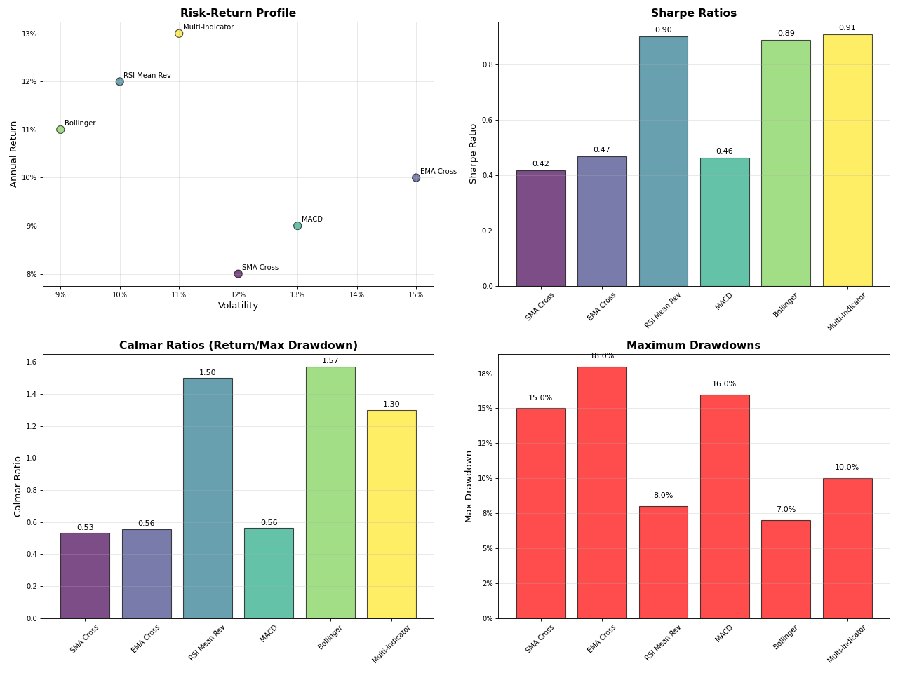
Risk-Adjusted Performance

import numpy as np
import matplotlib.pyplot as plt

# Simulate performance for different indicators
np.random.seed(42)

indicators = ['SMA Cross', 'EMA Cross', 'RSI Mean Rev', 'MACD', 'Bollinger', 'Multi-Indicator']

# Simulate annual returns and volatilities for each strategy
performance_data = {
    'SMA Cross': {'return': 0.08, 'volatility': 0.12, 'max_dd': 0.15},
    'EMA Cross': {'return': 0.10, 'volatility': 0.15, 'max_dd': 0.18},
    'RSI Mean Rev': {'return': 0.12, 'volatility': 0.10, 'max_dd': 0.08},
    'MACD': {'return': 0.09, 'volatility': 0.13, 'max_dd': 0.16},
    'Bollinger': {'return': 0.11, 'volatility': 0.09, 'max_dd': 0.07},
    'Multi-Indicator': {'return': 0.13, 'volatility': 0.11, 'max_dd': 0.10}
}

# Calculate risk-adjusted metrics
risk_free = 0.03
for strategy in performance_data:
    data = performance_data[strategy]
    data['sharpe'] = (data['return'] - risk_free) / data['volatility']
    data['calmar'] = data['return'] / data['max_dd']

# Create comparison chart
fig, ((ax1, ax2), (ax3, ax4)) = plt.subplots(2, 2, figsize=(16, 12))

strategies = list(performance_data.keys())
returns = [performance_data[s]['return'] for s in strategies]
volatilities = [performance_data[s]['volatility'] for s in strategies]
sharpes = [performance_data[s]['sharpe'] for s in strategies]
calmars = [performance_data[s]['calmar'] for s in strategies]

# Return vs Volatility
colors = plt.cm.viridis(np.linspace(0, 1, len(strategies)))
ax1.scatter(volatilities, returns, c=colors, s=100, alpha=0.7, edgecolors='black')
for i, strategy in enumerate(strategies):
    ax1.annotate(strategy, (volatilities[i], returns[i]),
                xytext=(5, 5), textcoords='offset points', fontsize=9)
ax1.set_xlabel('Volatility', fontsize=12)
ax1.set_ylabel('Annual Return', fontsize=12)
ax1.set_title('Risk-Return Profile', fontsize=14, fontweight='bold')
ax1.grid(True, alpha=0.3)
ax1.xaxis.set_major_formatter(plt.FuncFormatter(lambda x, p: f'{x:.0%}'))
ax1.yaxis.set_major_formatter(plt.FuncFormatter(lambda x, p: f'{x:.0%}'))

# Sharpe Ratios
bars1 = ax2.bar(strategies, sharpes, color=colors, alpha=0.7, edgecolor='black')
ax2.set_title('Sharpe Ratios', fontsize=14, fontweight='bold')
ax2.set_ylabel('Sharpe Ratio', fontsize=12)
ax2.tick_params(axis='x', rotation=45)
ax2.grid(True, alpha=0.3, axis='y')
for bar, value in zip(bars1, sharpes):
    ax2.text(bar.get_x() + bar.get_width()/2., bar.get_height() + 0.01,
            f'{value:.2f}', ha='center', va='bottom', fontsize=10)

# Calmar Ratios
bars2 = ax3.bar(strategies, calmars, color=colors, alpha=0.7, edgecolor='black')
ax3.set_title('Calmar Ratios (Return/Max Drawdown)', fontsize=14, fontweight='bold')
ax3.set_ylabel('Calmar Ratio', fontsize=12)
ax3.tick_params(axis='x', rotation=45)
ax3.grid(True, alpha=0.3, axis='y')
for bar, value in zip(bars2, calmars):
    ax3.text(bar.get_x() + bar.get_width()/2., bar.get_height() + 0.01,
            f'{value:.2f}', ha='center', va='bottom', fontsize=10)

# Risk metrics comparison
max_dds = [performance_data[s]['max_dd'] for s in strategies]
bars3 = ax4.bar(strategies, max_dds, color='red', alpha=0.7, edgecolor='black')
ax4.set_title('Maximum Drawdowns', fontsize=14, fontweight='bold')
ax4.set_ylabel('Max Drawdown', fontsize=12)
ax4.tick_params(axis='x', rotation=45)
ax4.grid(True, alpha=0.3, axis='y')
ax4.yaxis.set_major_formatter(plt.FuncFormatter(lambda x, p: f'{x:.0%}'))
for bar, value in zip(bars3, max_dds):
    ax4.text(bar.get_x() + bar.get_width()/2., bar.get_height() + 0.005,
            f'{value:.1%}', ha='center', va='bottom', fontsize=10)

plt.tight_layout()
plt.show()

Implementation Complexity

Implementation and Computational Requirements

Indicator	Complexity	CPU Usage	Memory Usage	Implementation Notes
SMA	Very Low	Very Low	Low	Simple rolling average
EMA	Low	Low	Very Low	Recursive calculation
RSI	Medium	Medium	Medium	Requires gain/loss tracking
MACD	Medium	Medium	Medium	Multiple EMA calculations
Bollinger Bands	Medium	Medium	Medium	SMA + standard deviation
Stochastic	Medium	Medium	Medium	Min/max lookback required
Williams %R	Medium	Medium	Medium	Similar to Stochastic
ATR	Medium	Medium	Medium	True range calculation
ADX	High	High	High	Complex directional calculations
Parabolic SAR	High	High	Medium	Acceleration factor logic
Ichimoku	Very High	High	High	Multiple components

Best Practices Summary

Parameter Selection: - Start with widely accepted defaults - Optimize for specific market conditions - Consider computational constraints - Account for data frequency

Signal Filtering: - Combine multiple timeframes - Use volume confirmation - Consider market regime - Apply risk management rules

Risk Management: - Always use stop losses - Position size appropriately - Diversify across strategies - Monitor correlation between signals

Backtesting Guidelines: - Use out-of-sample testing - Account for transaction costs - Include slippage estimates - Test across different market conditions - Avoid overfitting parameters