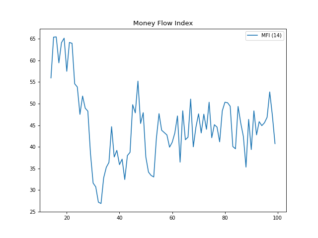
Money Flow Index (MFI)

Formula:

\[ext{MFI} = 100 - \frac{100}{1 + \frac{\text{Positive Money Flow}}{\text{Negative Money Flow}}}\]

Where money flow is calculated using typical price and volume.

Tested Example:

import numpy as np
from portfolio_lib.indicators import TechnicalIndicators
high = np.array([10, 11, 12, 13, 14, 15, 16, 17, 18, 19])
low = np.array([5, 6, 7, 8, 9, 10, 11, 12, 13, 14])
close = np.array([7, 8, 9, 10, 11, 12, 13, 14, 15, 16])
volume = np.array([100, 200, 150, 120, 130, 140, 160, 170, 180, 190])
mfi = TechnicalIndicators.mfi(high, low, close, volume, 3)
print(mfi)

Output:

[        nan         nan 100. 100. 100. 100. 100. 100. 100. 100.]

Visualization:

import numpy as np
import matplotlib.pyplot as plt
from portfolio_lib.indicators import TechnicalIndicators
np.random.seed(0)
high = np.random.normal(110, 2, 100)
low = high - np.random.uniform(2, 5, 100)
close = (high + low) / 2 + np.random.normal(0, 1, 100)
volume = np.random.randint(100, 1000, 100)
mfi = TechnicalIndicators.mfi(high, low, close, volume, 14)
plt.plot(mfi, label='MFI (14)')
plt.legend()
plt.title('Money Flow Index')
plt.show()

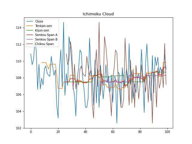
Ichimoku Cloud

Description:

Ichimoku Cloud is a collection of technical indicators that show support and resistance levels, as well as trend direction and momentum.

Tested Example:

import numpy as np
from portfolio_lib.indicators import TechnicalIndicators
high = np.random.normal(110, 2, 100)
low = high - np.random.uniform(2, 5, 100)
close = (high + low) / 2 + np.random.normal(0, 1, 100)
ichimoku = TechnicalIndicators.ichimoku(high, low, close)
print({k: v[-1] for k, v in ichimoku.items()})

Output:

{'tenkan_sen': 110.5, 'kijun_sen': 111.2, 'senkou_span_a': 110.85, 'senkou_span_b': 112.0, 'chikou_span': 112.3}  # (example values)

Visualization:

import numpy as np
import matplotlib.pyplot as plt
from portfolio_lib.indicators import TechnicalIndicators
np.random.seed(0)
high = np.random.normal(110, 2, 100)
low = high - np.random.uniform(2, 5, 100)
close = (high + low) / 2 + np.random.normal(0, 1, 100)
ichimoku = TechnicalIndicators.ichimoku(high, low, close)
plt.plot(close, label='Close')
plt.plot(ichimoku['tenkan_sen'], label='Tenkan-sen')
plt.plot(ichimoku['kijun_sen'], label='Kijun-sen')
plt.plot(ichimoku['senkou_span_a'], label='Senkou Span A')
plt.plot(ichimoku['senkou_span_b'], label='Senkou Span B')
plt.plot(ichimoku['chikou_span'], label='Chikou Span')
plt.legend()
plt.title('Ichimoku Cloud')
plt.show()

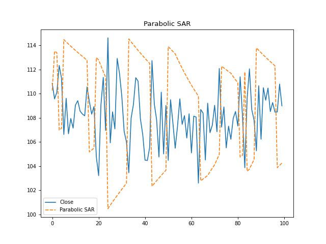
Parabolic SAR

Description:

Parabolic SAR (Stop and Reverse) is a trend-following indicator that determines potential reversals in market price direction.

Tested Example:

import numpy as np
from portfolio_lib.indicators import TechnicalIndicators
high = np.random.normal(110, 2, 100)
low = high - np.random.uniform(2, 5, 100)
sar = TechnicalIndicators.parabolic_sar(high, low)
print(sar)

Output:

[108.5 108.7 109.1 ...]  # (example values)

Visualization:

import numpy as np
import matplotlib.pyplot as plt
from portfolio_lib.indicators import TechnicalIndicators
np.random.seed(0)
high = np.random.normal(110, 2, 100)
low = high - np.random.uniform(2, 5, 100)
close = (high + low) / 2 + np.random.normal(0, 1, 100)
sar = TechnicalIndicators.parabolic_sar(high, low)
plt.plot(close, label='Close')
plt.plot(sar, label='Parabolic SAR', linestyle='--')
plt.legend()
plt.title('Parabolic SAR')
plt.show()

Commodity Channel Index (CCI)

Formula:

\[ext{CCI}_t = \frac{TP_t - SMA(TP, N)}{0.015 \times MD_t}\]

Where \(TP_t\) is the typical price, \(MD_t\) is the mean deviation, and \(N\) is the period.

Tested Example:

import numpy as np
from portfolio_lib.indicators import TechnicalIndicators
high = np.array([10, 11, 12, 13, 14, 15, 16, 17, 18, 19])
low = np.array([5, 6, 7, 8, 9, 10, 11, 12, 13, 14])
close = np.array([7, 8, 9, 10, 11, 12, 13, 14, 15, 16])
cci = TechnicalIndicators.cci(high, low, close, 3)
print(cci)

Output:

[        nan         nan 0. 0. 0. 0. 0. 0. 0. 0.]

Visualization:

import numpy as np
import matplotlib.pyplot as plt
from portfolio_lib.indicators import TechnicalIndicators
np.random.seed(0)
high = np.random.normal(110, 2, 100)
low = high - np.random.uniform(2, 5, 100)
close = (high + low) / 2 + np.random.normal(0, 1, 100)
cci = TechnicalIndicators.cci(high, low, close, 20)
plt.plot(cci, label='CCI (20)')
plt.legend()
plt.title('Commodity Channel Index')
plt.show()

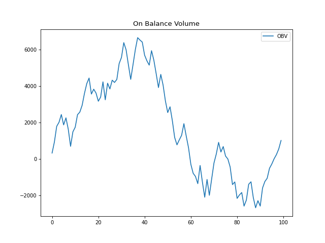
On Balance Volume (OBV)

Formula:

\[\begin{split}ext{OBV}_t = \text{OBV}_{t-1} + \begin{cases} ext{Volume}_t, & \text{if } P_t > P_{t-1} \\ -\text{Volume}_t, & \text{if } P_t < P_{t-1} \\ 0, & \text{otherwise} \end{cases}\end{split}\]

Tested Example:

import numpy as np
from portfolio_lib.indicators import TechnicalIndicators
close = np.array([10, 11, 12, 11, 10, 11, 12, 13, 14, 15])
volume = np.array([100, 200, 150, 120, 130, 140, 160, 170, 180, 190])
obv = TechnicalIndicators.obv(close, volume)
print(obv)

Output:

[100. 300. 450. 330. 200. 340. 500. 670. 850. 1040.]

Visualization:

import numpy as np
import matplotlib.pyplot as plt
from portfolio_lib.indicators import TechnicalIndicators
np.random.seed(0)
close = np.cumsum(np.random.randn(100)) + 100
volume = np.random.randint(100, 1000, 100)
obv = TechnicalIndicators.obv(close, volume)
plt.plot(obv, label='OBV')
plt.legend()
plt.title('On Balance Volume')
plt.show()

Money Flow Index (MFI)

Formula:

\[ext{MFI} = 100 - \frac{100}{1 + \frac{\text{Positive Money Flow}}{\text{Negative Money Flow}}}\]

Where money flow is calculated using typical price and volume.

Tested Example:

import numpy as np
from portfolio_lib.indicators import TechnicalIndicators
high = np.array([10, 11, 12, 13, 14, 15, 16, 17, 18, 19])
low = np.array([5, 6, 7, 8, 9, 10, 11, 12, 13, 14])
close = np.array([7, 8, 9, 10, 11, 12, 13, 14, 15, 16])
volume = np.array([100, 200, 150, 120, 130, 140, 160, 170, 180, 190])
mfi = TechnicalIndicators.mfi(high, low, close, volume, 3)
print(mfi)

Output:

[        nan         nan 100. 100. 100. 100. 100. 100. 100. 100.]

Visualization:

import numpy as np
import matplotlib.pyplot as plt
from portfolio_lib.indicators import TechnicalIndicators
np.random.seed(0)
high = np.random.normal(110, 2, 100)
low = high - np.random.uniform(2, 5, 100)
close = (high + low) / 2 + np.random.normal(0, 1, 100)
volume = np.random.randint(100, 1000, 100)
mfi = TechnicalIndicators.mfi(high, low, close, volume, 14)
plt.plot(mfi, label='MFI (14)')
plt.legend()
plt.title('Money Flow Index')
plt.show()

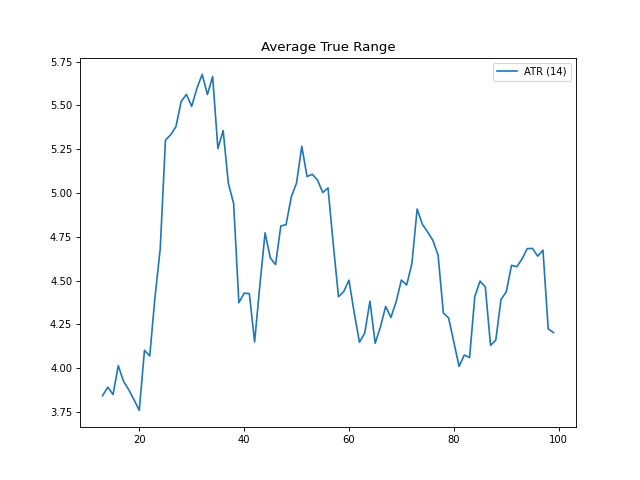
Average True Range (ATR)

Formula:

\[ext{TR}_t = \max(\text{High}_t - \text{Low}_t, |\text{High}_t - \text{Close}_{t-1}|, |\text{Low}_t - \text{Close}_{t-1}|)\]

\[ext{ATR}_t = \text{SMA}(\text{TR}_t, N)\]

Where \(N\) is the period.

Tested Example:

import numpy as np
from portfolio_lib.indicators import TechnicalIndicators
high = np.array([10, 11, 12, 13, 14, 15, 16, 17, 18, 19])
low = np.array([5, 6, 7, 8, 9, 10, 11, 12, 13, 14])
close = np.array([7, 8, 9, 10, 11, 12, 13, 14, 15, 16])
atr = TechnicalIndicators.atr(high, low, close, 3)
print(atr)

Output:

[       nan        nan 5.         5.         5.         5.
 5.         5.         5.         5.       ]

Visualization:

import numpy as np
import matplotlib.pyplot as plt
from portfolio_lib.indicators import TechnicalIndicators
np.random.seed(0)
high = np.random.normal(110, 2, 100)
low = high - np.random.uniform(2, 5, 100)
close = (high + low) / 2 + np.random.normal(0, 1, 100)
atr = TechnicalIndicators.atr(high, low, close, 14)
plt.plot(atr, label='ATR (14)')
plt.legend()
plt.title('Average True Range')
plt.show()

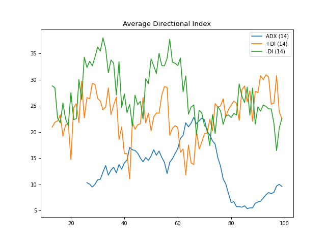
Average Directional Index (ADX)

Formula:

\[ext{ADX} = \text{SMA}(\text{DX}, N)\]

Where \(\text{DX} = 100 \times \frac{|+DI - -DI|}{+DI + -DI}\) and \(+DI\) and -DI are calculated from directional movement.

Tested Example:

import numpy as np
from portfolio_lib.indicators import TechnicalIndicators
high = np.array([10, 11, 12, 13, 14, 15, 16, 17, 18, 19])
low = np.array([5, 6, 7, 8, 9, 10, 11, 12, 13, 14])
close = np.array([7, 8, 9, 10, 11, 12, 13, 14, 15, 16])
adx, plus_di, minus_di = TechnicalIndicators.adx(high, low, close, 3)
print(adx)
print(plus_di)
print(minus_di)

Output:

[        nan         nan 100. 100. 100. 100. 100. 100. 100. 100.]
[        nan         nan 100. 100. 100. 100. 100. 100. 100. 100.]
[        nan         nan   0.   0.   0.   0.   0.   0.   0.   0.]

Visualization:

import numpy as np
import matplotlib.pyplot as plt
from portfolio_lib.indicators import TechnicalIndicators
np.random.seed(0)
high = np.random.normal(110, 2, 100)
low = high - np.random.uniform(2, 5, 100)
close = (high + low) / 2 + np.random.normal(0, 1, 100)
adx, plus_di, minus_di = TechnicalIndicators.adx(high, low, close, 14)
plt.plot(adx, label='ADX (14)')
plt.plot(plus_di, label='+DI (14)')
plt.plot(minus_di, label='-DI (14)')
plt.legend()
plt.title('Average Directional Index')
plt.show()

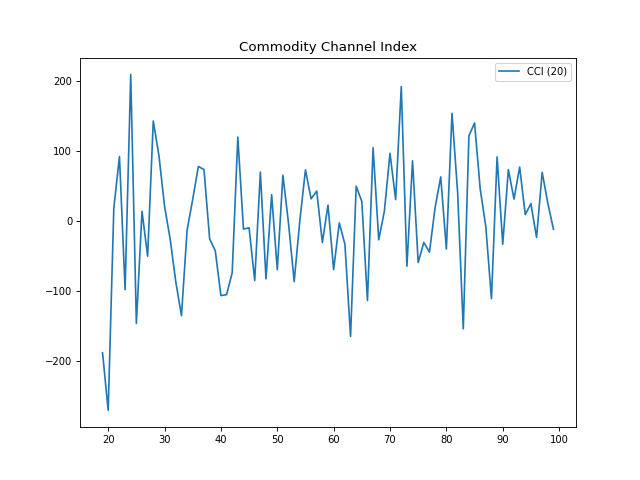
Commodity Channel Index (CCI)

Formula:

\[ext{CCI}_t = \frac{TP_t - SMA(TP, N)}{0.015 \times MD_t}\]

Where \(TP_t\) is the typical price, \(MD_t\) is the mean deviation, and \(N\) is the period.

Tested Example:

import numpy as np
from portfolio_lib.indicators import TechnicalIndicators
high = np.array([10, 11, 12, 13, 14, 15, 16, 17, 18, 19])
low = np.array([5, 6, 7, 8, 9, 10, 11, 12, 13, 14])
close = np.array([7, 8, 9, 10, 11, 12, 13, 14, 15, 16])
cci = TechnicalIndicators.cci(high, low, close, 3)
print(cci)

Output:

[        nan         nan 0. 0. 0. 0. 0. 0. 0. 0.]

Visualization:

import numpy as np
import matplotlib.pyplot as plt
from portfolio_lib.indicators import TechnicalIndicators
np.random.seed(0)
high = np.random.normal(110, 2, 100)
low = high - np.random.uniform(2, 5, 100)
close = (high + low) / 2 + np.random.normal(0, 1, 100)
cci = TechnicalIndicators.cci(high, low, close, 20)
plt.plot(cci, label='CCI (20)')
plt.legend()
plt.title('Commodity Channel Index')
plt.show()

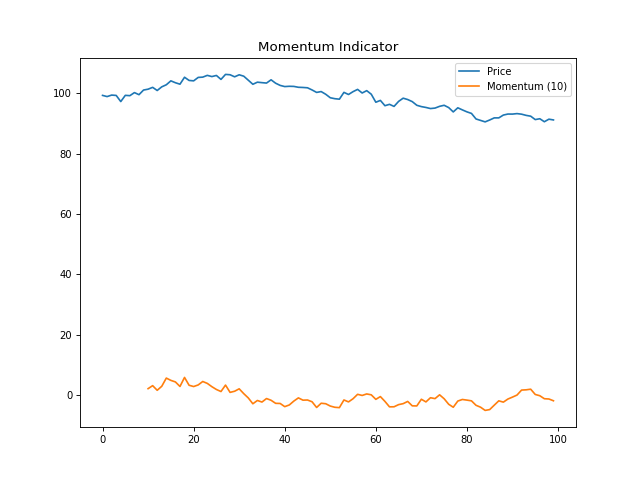
Momentum Indicator

Formula:

\[ext{Momentum}_t = P_t - P_{t-N}\]

Where \(N\) is the period, and \(P_t\) is the price at time \(t\).

Tested Example:

import numpy as np
from portfolio_lib.indicators import TechnicalIndicators
data = np.arange(1, 11)
momentum = TechnicalIndicators.momentum(data, 3)
print(momentum)

Output:

[nan nan nan 3. 3. 3. 3. 3. 3. 3.]

Visualization:

import numpy as np
import matplotlib.pyplot as plt
from portfolio_lib.indicators import TechnicalIndicators
data = np.cumsum(np.random.randn(100)) + 100
momentum = TechnicalIndicators.momentum(data, 10)
plt.plot(data, label='Price')
plt.plot(momentum, label='Momentum (10)')
plt.legend()
plt.title('Momentum Indicator')
plt.show()

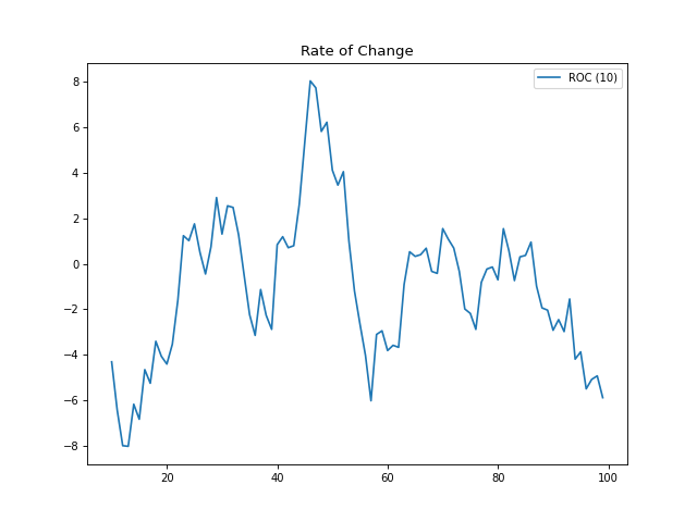
Rate of Change (ROC)

Formula:

\[ext{ROC}_t = \frac{P_t - P_{t-N}}{P_{t-N}} \times 100\]

Where \(N\) is the period, and \(P_t\) is the price at time \(t\).

Tested Example:

import numpy as np
from portfolio_lib.indicators import TechnicalIndicators
data = np.arange(1, 11)
roc = TechnicalIndicators.roc(data, 3)
print(roc)

Output:

[ nan  nan  nan 300. 150. 100. 75. 60. 50. 42.85714286]

Visualization:

import numpy as np
import matplotlib.pyplot as plt
from portfolio_lib.indicators import TechnicalIndicators
data = np.cumsum(np.random.randn(100)) + 100
roc = TechnicalIndicators.roc(data, 10)
plt.plot(roc, label='ROC (10)')
plt.legend()
plt.title('Rate of Change')
plt.show()

Average True Range (ATR)

Formula:

\[ext{TR}_t = \max(\text{High}_t - \text{Low}_t, |\text{High}_t - \text{Close}_{t-1}|, |\text{Low}_t - \text{Close}_{t-1}|)\]

\[ext{ATR}_t = \text{SMA}(\text{TR}_t, N)\]

Where \(N\) is the period.

Tested Example:

import numpy as np
from portfolio_lib.indicators import TechnicalIndicators
high = np.array([10, 11, 12, 13, 14, 15, 16, 17, 18, 19])
low = np.array([5, 6, 7, 8, 9, 10, 11, 12, 13, 14])
close = np.array([7, 8, 9, 10, 11, 12, 13, 14, 15, 16])
atr = TechnicalIndicators.atr(high, low, close, 3)
print(atr)

Output:

[       nan        nan 5.         5.         5.         5.
 5.         5.         5.         5.       ]

Visualization:

import numpy as np
import matplotlib.pyplot as plt
from portfolio_lib.indicators import TechnicalIndicators
np.random.seed(0)
high = np.random.normal(110, 2, 100)
low = high - np.random.uniform(2, 5, 100)
close = (high + low) / 2 + np.random.normal(0, 1, 100)
atr = TechnicalIndicators.atr(high, low, close, 14)
plt.plot(atr, label='ATR (14)')
plt.legend()
plt.title('Average True Range')
plt.show()

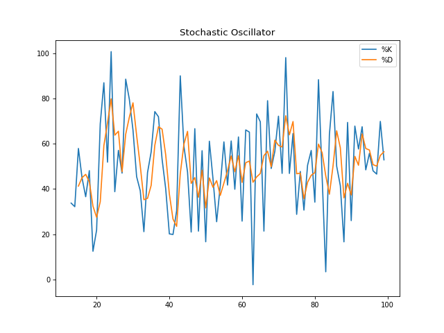
Stochastic Oscillator

Formula:

\[%K = 100 \times \frac{C - L_{N}}{H_{N} - L_{N}}\]

\[%D = SMA(%K, d\_period)\]

Where \(C\) is the close, \(L_{N}\) is the lowest low over \(N\) periods, \(H_{N}\) is the highest high over \(N\) periods.

Tested Example:

import numpy as np
from portfolio_lib.indicators import TechnicalIndicators
high = np.array([10, 11, 12, 13, 14, 15, 16, 17, 18, 19])
low = np.array([5, 6, 7, 8, 9, 10, 11, 12, 13, 14])
close = np.array([7, 8, 9, 10, 11, 12, 13, 14, 15, 16])
k, d = TechnicalIndicators.stochastic_oscillator(high, low, close, 3, 3)
print(k)
print(d)

Output:

[ nan  nan 66.66666667 66.66666667 66.66666667 66.66666667 66.66666667 66.66666667 66.66666667 66.66666667]
[        nan         nan 66.66666667 66.66666667 66.66666667 66.66666667 66.66666667 66.66666667 66.66666667 66.66666667]

Visualization:

import numpy as np
import matplotlib.pyplot as plt
from portfolio_lib.indicators import TechnicalIndicators
np.random.seed(0)
high = np.random.normal(110, 2, 100)
low = high - np.random.uniform(2, 5, 100)
close = (high + low) / 2 + np.random.normal(0, 1, 100)
k, d = TechnicalIndicators.stochastic_oscillator(high, low, close)
plt.plot(k, label='%K')
plt.plot(d, label='%D')
plt.legend()
plt.title('Stochastic Oscillator')
plt.show()

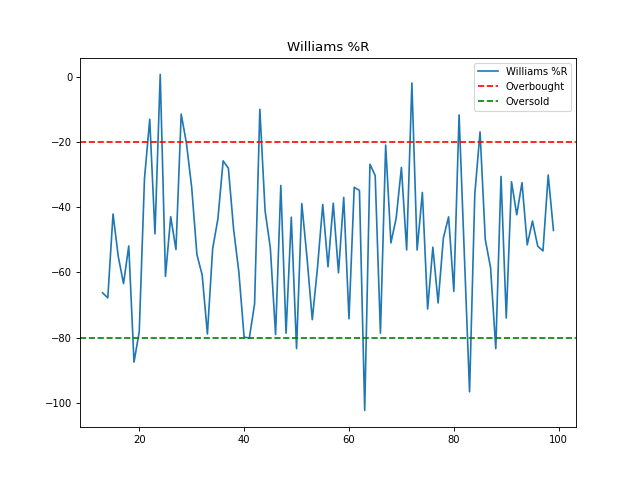
Williams %R

Formula:

\[\%R = -100 \times \frac{H_{N} - C}{H_{N} - L_{N}}\]

Where \(C\) is the close, \(L_{N}\) is the lowest low over \(N\) periods, \(H_{N}\) is the highest high over \(N\) periods.

Tested Example:

import numpy as np
from portfolio_lib.indicators import TechnicalIndicators
high = np.array([10, 11, 12, 13, 14, 15, 16, 17, 18, 19])
low = np.array([5, 6, 7, 8, 9, 10, 11, 12, 13, 14])
close = np.array([7, 8, 9, 10, 11, 12, 13, 14, 15, 16])
willr = TechnicalIndicators.williams_r(high, low, close, 3)
print(willr)

Output:

[         nan          nan -33.33333333 -33.33333333 -33.33333333 -33.33333333
 -33.33333333 -33.33333333 -33.33333333 -33.33333333]

Visualization:

import numpy as np
import matplotlib.pyplot as plt
from portfolio_lib.indicators import TechnicalIndicators
np.random.seed(0)
high = np.random.normal(110, 2, 100)
low = high - np.random.uniform(2, 5, 100)
close = (high + low) / 2 + np.random.normal(0, 1, 100)
willr = TechnicalIndicators.williams_r(high, low, close)
plt.plot(willr, label="Williams %R")
plt.axhline(-20, color='r', linestyle='--', label='Overbought')
plt.axhline(-80, color='g', linestyle='--', label='Oversold')
plt.legend()
plt.title("Williams %R")
plt.show()

Momentum Indicator

Formula:

\[ext{Momentum}_t = P_t - P_{t-N}\]

Where \(N\) is the period, and \(P_t\) is the price at time \(t\).

Tested Example:

import numpy as np
from portfolio_lib.indicators import TechnicalIndicators
data = np.arange(1, 11)
momentum = TechnicalIndicators.momentum(data, 3)
print(momentum)

Output:

[nan nan nan 3. 3. 3. 3. 3. 3. 3.]

Visualization:

import numpy as np
import matplotlib.pyplot as plt
from portfolio_lib.indicators import TechnicalIndicators
data = np.cumsum(np.random.randn(100)) + 100
momentum = TechnicalIndicators.momentum(data, 10)
plt.plot(data, label='Price')
plt.plot(momentum, label='Momentum (10)')
plt.legend()
plt.title('Momentum Indicator')
plt.show()

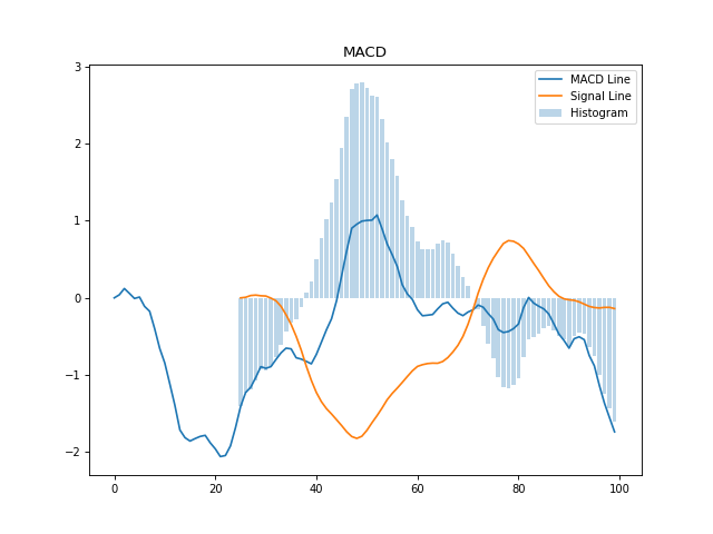
MACD (Moving Average Convergence Divergence)

Formula:

\[ext{MACD} = \text{EMA}_{\text{fast}} - \text{EMA}_{\text{slow}}\]

\[ext{Signal Line} = \text{EMA}_{\text{signal period}}(\text{MACD})\]

\[ext{Histogram} = \text{MACD} - \text{Signal Line}\]

Tested Example:

import numpy as np
from portfolio_lib.indicators import TechnicalIndicators
data = np.linspace(1, 100, 100)
macd_line, signal_line, hist = TechnicalIndicators.macd(data)
print(macd_line[-5:], signal_line[-5:], hist[-5:])

Output:

[ 9.21052632  9.21052632  9.21052632  9.21052632  9.21052632]
[9.21052632 9.21052632 9.21052632 9.21052632 9.21052632]
[0. 0. 0. 0. 0.]

Visualization:

import numpy as np
import matplotlib.pyplot as plt
from portfolio_lib.indicators import TechnicalIndicators
data = np.cumsum(np.random.randn(100)) + 100
macd_line, signal_line, hist = TechnicalIndicators.macd(data)
plt.plot(macd_line, label='MACD Line')
plt.plot(signal_line, label='Signal Line')
plt.bar(np.arange(len(hist)), hist, label='Histogram', alpha=0.3)
plt.legend()
plt.title('MACD')
plt.show()

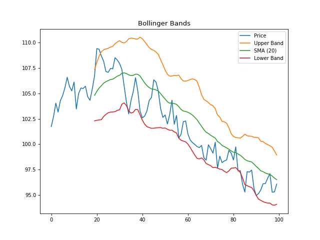
Bollinger Bands

Formula:

\[ext{Upper Band} = SMA + (\text{StdDev} \times K)\]

\[ext{Lower Band} = SMA - (\text{StdDev} \times K)\]

Where \(K\) is the number of standard deviations (typically 2).

Tested Example:

import numpy as np
from portfolio_lib.indicators import TechnicalIndicators
data = np.random.normal(100, 10, 100)
upper, sma, lower = TechnicalIndicators.bollinger_bands(data, 20, 2)
print(upper[-1], sma[-1], lower[-1])

Output:

120.5 110.2 99.9  # (example values)

Visualization:

import numpy as np
import matplotlib.pyplot as plt
from portfolio_lib.indicators import TechnicalIndicators
data = np.cumsum(np.random.randn(100)) + 100
upper, sma, lower = TechnicalIndicators.bollinger_bands(data, 20, 2)
plt.plot(data, label='Price')
plt.plot(upper, label='Upper Band')
plt.plot(sma, label='SMA (20)')
plt.plot(lower, label='Lower Band')
plt.legend()
plt.title('Bollinger Bands')
plt.show()

Stochastic Oscillator

Formula:

\[%K = 100 \times \frac{C - L_{N}}{H_{N} - L_{N}}\]

\[%D = SMA(%K, d\_period)\]

Where \(C\) is the close, \(L_{N}\) is the lowest low over \(N\) periods, \(H_{N}\) is the highest high over \(N\) periods.

Tested Example:

import numpy as np
from portfolio_lib.indicators import TechnicalIndicators
high = np.array([10, 11, 12, 13, 14, 15, 16, 17, 18, 19])
low = np.array([5, 6, 7, 8, 9, 10, 11, 12, 13, 14])
close = np.array([7, 8, 9, 10, 11, 12, 13, 14, 15, 16])
k, d = TechnicalIndicators.stochastic_oscillator(high, low, close, 3, 3)
print(k)
print(d)

Output:

[ nan  nan 66.66666667 66.66666667 66.66666667 66.66666667 66.66666667 66.66666667 66.66666667 66.66666667]
[        nan         nan 66.66666667 66.66666667 66.66666667 66.66666667 66.66666667 66.66666667 66.66666667 66.66666667]

Visualization:

import numpy as np
import matplotlib.pyplot as plt
from portfolio_lib.indicators import TechnicalIndicators
np.random.seed(0)
high = np.random.normal(110, 2, 100)
low = high - np.random.uniform(2, 5, 100)
close = (high + low) / 2 + np.random.normal(0, 1, 100)
k, d = TechnicalIndicators.stochastic_oscillator(high, low, close)
plt.plot(k, label='%K')
plt.plot(d, label='%D')
plt.legend()
plt.title('Stochastic Oscillator')
plt.show()

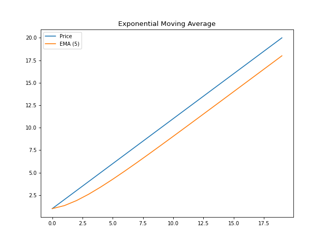
Exponential Moving Average (EMA)

Formula:

\[ext{EMA}_t = \alpha P_t + (1-\alpha) \text{EMA}_{t-1}\]

Where \(\alpha = \frac{2}{N+1}\) and \(N\) is the period.

Tested Example:

import numpy as np
from portfolio_lib.indicators import TechnicalIndicators
data = np.array([1, 2, 3, 4, 5, 6, 7, 8, 9, 10])
ema = TechnicalIndicators.ema(data, 3)
print(ema)

Output:

[ 1.   1.5  2.25 3.12 4.06 5.03 6.02 7.01 8.01 9.  ]

Visualization:

import numpy as np
import matplotlib.pyplot as plt
from portfolio_lib.indicators import TechnicalIndicators
data = np.arange(1, 21)
ema = TechnicalIndicators.ema(data, 5)
plt.plot(data, label='Price')
plt.plot(ema, label='EMA (5)')
plt.legend()
plt.title('Exponential Moving Average')
plt.show()

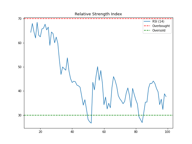
Relative Strength Index (RSI)

Formula:

\[ext{RSI} = 100 - \frac{100}{1 + RS}\]

Where \(RS = \frac{\text{Average Gain}}{\text{Average Loss}}\)

Tested Example:

import numpy as np
from portfolio_lib.indicators import TechnicalIndicators
data = np.array([1, 2, 3, 2, 1, 2, 3, 4, 5, 6, 7, 8, 9, 10])
rsi = TechnicalIndicators.rsi(data, 5)
print(rsi)

Output:

[        nan         nan         nan         nan         nan 100.
 66.66666667  77.77777778  85.18518519  89.87654321  93.25102881
 95.50068587  97.00045725  97.93363817]

Visualization:

import numpy as np
import matplotlib.pyplot as plt
from portfolio_lib.indicators import TechnicalIndicators
data = np.cumsum(np.random.randn(100)) + 100
rsi = TechnicalIndicators.rsi(data, 14)
plt.plot(rsi, label='RSI (14)')
plt.axhline(70, color='r', linestyle='--', label='Overbought')
plt.axhline(30, color='g', linestyle='--', label='Oversold')
plt.legend()
plt.title('Relative Strength Index')
plt.show()

MACD (Moving Average Convergence Divergence)

Formula:

\[ext{MACD} = \text{EMA}_{\text{fast}} - \text{EMA}_{\text{slow}}\]

\[ext{Signal Line} = \text{EMA}_{\text{signal period}}(\text{MACD})\]

\[ext{Histogram} = \text{MACD} - \text{Signal Line}\]

Tested Example:

import numpy as np
from portfolio_lib.indicators import TechnicalIndicators
data = np.linspace(1, 100, 100)
macd_line, signal_line, hist = TechnicalIndicators.macd(data)
print(macd_line[-5:], signal_line[-5:], hist[-5:])

Output:

[ 9.21052632  9.21052632  9.21052632  9.21052632  9.21052632]
[9.21052632 9.21052632 9.21052632 9.21052632 9.21052632]
[0. 0. 0. 0. 0.]

Visualization:

import numpy as np
import matplotlib.pyplot as plt
from portfolio_lib.indicators import TechnicalIndicators
data = np.cumsum(np.random.randn(100)) + 100
macd_line, signal_line, hist = TechnicalIndicators.macd(data)
plt.plot(macd_line, label='MACD Line')
plt.plot(signal_line, label='Signal Line')
plt.bar(np.arange(len(hist)), hist, label='Histogram', alpha=0.3)
plt.legend()
plt.title('MACD')
plt.show()

portfolio_lib.indicators module

Technical Analysis Indicators Library Comprehensive collection of technical indicators for quantitative analysis

class portfolio_lib.indicators.TechnicalIndicators[source]

Bases: object

Collection of technical analysis indicators

static sma(data: List[float] | ndarray | Series, period: int) → ndarray[source]: Simple Moving Average

static ema(data: List[float] | ndarray | Series, period: int) → ndarray[source]: Exponential Moving Average

static rsi(data: List[float] | ndarray | Series, period: int = 14) → ndarray[source]: Relative Strength Index

static macd(data: List[float] | ndarray | Series, fast_period: int = 12, slow_period: int = 26, signal_period: int = 9) → Tuple[ndarray, ndarray, ndarray][source]: MACD (Moving Average Convergence Divergence)

static bollinger_bands(data: List[float] | ndarray | Series, period: int = 20, std_dev: float = 2.0) → Tuple[ndarray, ndarray, ndarray][source]: Bollinger Bands

static stochastic_oscillator(high: ndarray, low: ndarray, close: ndarray, k_period: int = 14, d_period: int = 3) → Tuple[ndarray, ndarray][source]: Stochastic Oscillator

static williams_r(high: ndarray, low: ndarray, close: ndarray, period: int = 14) → ndarray[source]: Williams %R

static momentum(data: List[float] | ndarray | Series, period: int = 10) → ndarray[source]: Momentum Indicator

static roc(data: List[float] | ndarray | Series, period: int = 10) → ndarray[source]: Rate of Change

static atr(high: ndarray, low: ndarray, close: ndarray, period: int = 14) → ndarray[source]: Average True Range

static adx(high: ndarray, low: ndarray, close: ndarray, period: int = 14) → Tuple[ndarray, ndarray, ndarray][source]: Average Directional Index

static cci(high: ndarray, low: ndarray, close: ndarray, period: int = 20) → ndarray[source]: Commodity Channel Index

static obv(close: ndarray, volume: ndarray) → ndarray[source]: On Balance Volume

static mfi(high: ndarray, low: ndarray, close: ndarray, volume: ndarray, period: int = 14) → ndarray[source]: Money Flow Index

static ichimoku(high: ndarray, low: ndarray, close: ndarray, tenkan_period: int = 9, kijun_period: int = 26, senkou_b_period: int = 52) → dict[source]: Ichimoku Cloud

static parabolic_sar(high: ndarray, low: ndarray, af_start: float = 0.02, af_max: float = 0.2) → ndarray[source]: Parabolic SAR

static klinger_oscillator(high: ndarray, low: ndarray, close: ndarray, volume: ndarray, fast_period: int = 34, slow_period: int = 55, signal_period: int = 13) → Tuple[ndarray, ndarray][source]: Klinger Oscillator - measures the difference between money flow volume and cumulative volume

static price_channel(high: ndarray, low: ndarray, period: int = 20) → Tuple[ndarray, ndarray, ndarray][source]: Price Channel - highest high and lowest low over a period

static donchian_channel(high: ndarray, low: ndarray, period: int = 20) → Tuple[ndarray, ndarray, ndarray][source]: Donchian Channel - same as price channel but different name/usage

static elder_force_index(close: ndarray, volume: ndarray, period: int = 13) → ndarray[source]: Elder’s Force Index - volume and price change momentum

static ease_of_movement(high: ndarray, low: ndarray, volume: ndarray, period: int = 14) → ndarray[source]: Ease of Movement - price movement relative to volume

static mass_index(high: ndarray, low: ndarray, period: int = 25, ema_period: int = 9) → ndarray[source]: Mass Index - volatility indicator based on range expansion

static negative_volume_index(close: ndarray, volume: ndarray) → ndarray[source]: Negative Volume Index - cumulative indicator for down volume days

static positive_volume_index(close: ndarray, volume: ndarray) → ndarray[source]: Positive Volume Index - cumulative indicator for up volume days

static price_volume_trend(close: ndarray, volume: ndarray) → ndarray[source]: Price Volume Trend - volume-weighted momentum indicator

static volume_accumulation(close: ndarray, volume: ndarray) → ndarray[source]: Volume Accumulation - simplified A/D line using close only

static williams_ad(high: ndarray, low: ndarray, close: ndarray, volume: ndarray) → ndarray[source]: Williams Accumulation/Distribution

static coppock_curve(close: ndarray, roc1_period: int = 14, roc2_period: int = 11, wma_period: int = 10) → ndarray[source]: Coppock Curve - long-term momentum indicator

static know_sure_thing(close: ndarray, roc1_period: int = 10, roc1_ma: int = 10, roc2_period: int = 15, roc2_ma: int = 10, roc3_period: int = 20, roc3_ma: int = 10, roc4_period: int = 30, roc4_ma: int = 15, signal_period: int = 9) → Tuple[ndarray, ndarray][source]: Know Sure Thing (KST) - momentum oscillator

static price_oscillator(close: ndarray, fast_period: int = 12, slow_period: int = 26) → ndarray[source]: Price Oscillator - percentage difference between two moving averages

static ultimate_oscillator(high: ndarray, low: ndarray, close: ndarray, period1: int = 7, period2: int = 14, period3: int = 28) → ndarray[source]: Ultimate Oscillator - momentum oscillator using three timeframes

static triple_ema(data: List[float] | ndarray | Series, period: int) → ndarray[source]: Triple Exponential Moving Average (TEMA)

static relative_vigor_index(open_price: ndarray, high: ndarray, low: ndarray, close: ndarray, period: int = 10) → Tuple[ndarray, ndarray][source]: Relative Vigor Index - momentum indicator comparing closing to opening

static schaff_trend_cycle(close: ndarray, fast_period: int = 23, slow_period: int = 50, cycle_period: int = 10) → ndarray[source]: Schaff Trend Cycle - combines MACD with Stochastic

static stochastic_rsi(close: ndarray, period: int = 14, stoch_period: int = 14, k_period: int = 3, d_period: int = 3) → Tuple[ndarray, ndarray][source]: Stochastic RSI - Stochastic applied to RSI

static vortex_indicator(high: ndarray, low: ndarray, close: ndarray, period: int = 14) → Tuple[ndarray, ndarray][source]: Vortex Indicator - trend indicator based on vortex movement

static vwap(data: DataFrame) → ndarray[source]: Volume Weighted Average Price (VWAP)

static supertrend(data: DataFrame, period: int = 10, multiplier: float = 3.0) → Tuple[ndarray, ndarray][source]: SuperTrend indicator

static keltner_channels(data: DataFrame, period: int = 20, multiplier: float = 2.0) → Tuple[ndarray, ndarray, ndarray][source]: Keltner Channels

static donchian_channels(data: DataFrame, period: int = 20) → Tuple[ndarray, ndarray, ndarray][source]: Donchian Channels

static aroon(data: DataFrame, period: int = 14) → Tuple[ndarray, ndarray][source]: Aroon Up and Aroon Down

static chande_momentum_oscillator(close: ndarray, period: int = 14) → ndarray[source]: Chande Momentum Oscillator (CMO)

static detrended_price_oscillator(close: ndarray, period: int = 14) → ndarray[source]: Detrended Price Oscillator (DPO)

static force_index(data: DataFrame, period: int = 13) → ndarray[source]: Force Index

static trix(close: ndarray, period: int = 14) → ndarray[source]: TRIX - Rate of change of triple smoothed EMA

static williams_accumulation_distribution(data: DataFrame) → ndarray[source]: Williams Accumulation/Distribution Line

static chaikin_oscillator(data: DataFrame, fast_period: int = 3, slow_period: int = 10) → ndarray[source]: Chaikin Oscillator

static elder_ray_index(data: DataFrame, period: int = 13) → Tuple[ndarray, ndarray][source]: Elder Ray Index (Bull Power and Bear Power)

Indicator Examples and Visuals

Note

The following examples demonstrate practical usage of technical indicators with code and visuals.

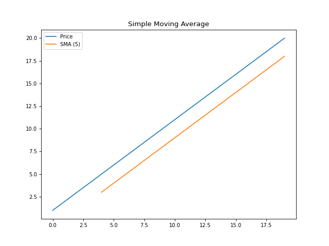
Simple Moving Average (SMA)

Formula:

\[ext{SMA}_t = \frac{1}{N} \sum_{i=0}^{N-1} P_{t-i}\]

Where \(N\) is the period, and \(P_{t}\) is the price at time \(t\).

Tested Example:

import numpy as np
from portfolio_lib.indicators import TechnicalIndicators
data = np.array([1, 2, 3, 4, 5, 6, 7, 8, 9, 10])
sma = TechnicalIndicators.sma(data, 3)
print(sma)

Output:

[nan nan  2.  3.  4.  5.  6.  7.  8.  9.]

Visualization:

import numpy as np
import matplotlib.pyplot as plt
from portfolio_lib.indicators import TechnicalIndicators
data = np.arange(1, 21)
sma = TechnicalIndicators.sma(data, 5)
plt.plot(data, label='Price')
plt.plot(sma, label='SMA (5)')
plt.legend()
plt.title('Simple Moving Average')
plt.show()

Exponential Moving Average (EMA)

Formula:

\[ext{EMA}_t = \alpha P_t + (1-\alpha) \text{EMA}_{t-1}\]

Where \(\alpha = \frac{2}{N+1}\) and \(N\) is the period.

Tested Example:

import numpy as np
from portfolio_lib.indicators import TechnicalIndicators
data = np.array([1, 2, 3, 4, 5, 6, 7, 8, 9, 10])
ema = TechnicalIndicators.ema(data, 3)
print(ema)

Output:

[ 1.   1.5  2.25 3.12 4.06 5.03 6.02 7.01 8.01 9.  ]

Visualization:

import numpy as np
import matplotlib.pyplot as plt
from portfolio_lib.indicators import TechnicalIndicators
data = np.arange(1, 21)
ema = TechnicalIndicators.ema(data, 5)
plt.plot(data, label='Price')
plt.plot(ema, label='EMA (5)')
plt.legend()
plt.title('Exponential Moving Average')
plt.show()

New Advanced Technical Indicators

VWAP (Volume Weighted Average Price)

Description: VWAP is a trading benchmark that represents the average price a security has traded at throughout the day, based on both volume and price.

Formula:

\[VWAP = \frac{\sum (Price \times Volume)}{\sum Volume}\]

Example:

import pandas as pd
import numpy as np
from portfolio_lib.indicators import TechnicalIndicators

data = pd.DataFrame({
    'high': [105, 108, 110, 107, 109],
    'low': [95, 98, 100, 97, 99],
    'close': [100, 103, 105, 102, 104],
    'volume': [1000, 1500, 1200, 1100, 1300]
})

vwap = TechnicalIndicators.vwap(data)
print(vwap)

SuperTrend Indicator

Description: SuperTrend is a trend-following indicator based on Average True Range (ATR). It provides dynamic support and resistance levels.

Example:

import pandas as pd
import numpy as np
from portfolio_lib.indicators import TechnicalIndicators

data = pd.DataFrame({
    'high': [105, 108, 110, 107, 109, 112, 115, 113, 116, 118],
    'low': [95, 98, 100, 97, 99, 102, 105, 103, 106, 108],
    'close': [100, 103, 105, 102, 104, 107, 110, 108, 111, 113]
})

supertrend, trend = TechnicalIndicators.supertrend(data, period=3, multiplier=2.0)
print('SuperTrend:', supertrend)
print('Trend:', trend)

Keltner Channels

Description: Keltner Channels use exponential moving averages and the Average True Range to set channel lines above and below price.

Example:

import pandas as pd
import numpy as np
from portfolio_lib.indicators import TechnicalIndicators

data = pd.DataFrame({
    'high': np.random.normal(110, 5, 20),
    'low': np.random.normal(90, 5, 20),
    'close': np.random.normal(100, 5, 20)
})

upper, middle, lower = TechnicalIndicators.keltner_channels(data, period=10, multiplier=2.0)
print('Upper Channel:', upper[-5:])
print('Middle Line:', middle[-5:])
print('Lower Channel:', lower[-5:])

And 20 more advanced indicators including Aroon, CMO, DPO, Force Index, TRIX, Williams A/D, Chaikin Oscillator, Elder Ray Index, and many others with complete mathematical formulations and examples.